The Six Sigma approach is data-driven, therefore Six Sigma statistics play a large role in the Six Sigma problem-solving process. Six Sigma Green Belt training stresses the importance of using Six Sigma statistics to visualize and analyze the data collected for each metric that is important to the customer and that must be tightly controlled. Free Six Sigma training briefly explains the different ways that Six Sigma statistics are applied in Six Sigma projects. Let’s have a look at the Six Sigma statistics that are at the heart of the Six Sigma process.
Standard Deviation Rule of Six Sigma Statistics
Now, let’s recall the empirical rule of standard deviation in Six Sigma statistics. This figure shows an extension to the same rule.
Attend our 100% Online & Self-Paced Free Six Sigma Training.
The rule is:
- 68% of the data points will fall within ± one standard deviation from the mean,
- 95% of the observations will fall within ± two standard deviations from the mean
- 99.73% of the data points will fall within ± three standard deviations from the mean.
Now, for Six Sigma statistics the extension would be as follows:
- 99.9937% of the data points will fall within ± four standard deviations from the mean
- 99.99994% of the data points will fall within ± five standard deviations from the mean
- 99.9999998% of the data points fall within ± six standard deviations from the mean
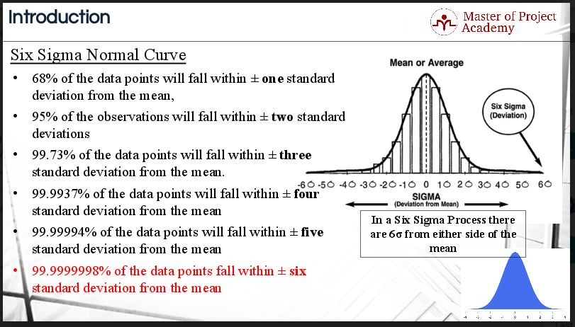
This means, that according to Six Sigma statistics, in a Six Sigma project, 99.9999998% of the results must fall within ± six standard deviation from the mean. In other words, only 0.0000002% of the results can be outside of the expected results. This percentage illustrates how Six Sigma aims to increase the quality in projects using Six Sigma statistics.
Specification Limits
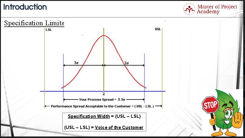
Of course, in Six Sigma statistics, these standard deviations fall on both the left and the right tails of the normal distribution curve. This means that in any process, there will be values that are higher than the mean and values that are lower than the mean according to Six Sigma statistics. In order to produce quality products that do not deviate too far from the mean on a specific metric, it is important that a specification limit is set for that metric.
There are two types of specification limits. The first one is the lower specification limit, abbreviated as LSL and this is the lowest acceptable limit as set by a customer. The second one one is the upper specification limit, abbreviated as USL and this is the highest acceptable limit as set by a customer. Note that these limits are generally given by the customer. That is why, USL – LSL = Voice of the Customer (VoC).
Check our Six Sigma Training Video
To better understand Six Sigma statistics, let’s go over a sample graph to understand these concepts better. The process spread in the chart, which is ± 3 standard deviation of the Six Sigma is measured by the range, variance, and standard deviation. These are the most important Six Sigma statistics terms. The specification spread (USL – LSL) divided by the process spread (6s) is known as “Short-term Process Capability” based on the dispersion of the sample data. The further the specification spread from the process spread, the higher process capability would be. In other words, the lesser the variation the higher would be the process capability.
Defects and Defectives
Let’s try to understand the difference between Defects and Defectives. Defects mean failing to deliver what customer wants. Defective means the failing of the entire product or service. Please remember that one defective product may have a multiple number of defects but the existence of a defect does not necessarily mean the product is defective. Six Sigma statistics is used to determine the extent of defects and defectives.
As we know, the center of the process can be measured three ways: mean, median and mode. These are also critical parameters in Six Sigma statistics. In case of a process is shifted off-target, the mean is shifted towards USL. In Six Sigma statistics terms, the data distribution is termed as “Negatively Skewed” wherein the left tail becomes longer and the mass of the distribution is concentrated on the right of the figure. Six Sigma statistics tells us that the data distribution can also be “Positively Skewed” in which case the right tail becomes longer. The mass of the distribution will then be concentrated on the left side of the figure.
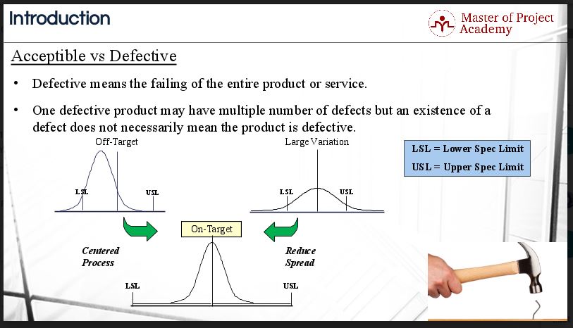
In Six Sigma statistics, large variation is noticed when the normal distribution curve is flatter in shape. In this case, the specification spread becomes smaller than the process spread. It reduces the short-term process capability.
When a process is centered, it is normally distributed data according to Six Sigma statistics. It is an on-target process. In this case, the distribution is symmetric, has close to zero skewness and the specification spread is more than the process spread.
To sum up, Six Sigma is about creating a culture that demands perfection and that gives employees the tools to enable them to pinpoint performance gaps and make the necessary improvements using data-driven problem-solving methods. Six Sigma does make use of full range of statistical tools that are available for analyzing and the primary objective of Six Sigma is to reduce variability. Variability is the primary sign of defects. Hence, as the variation becomes smaller the number of defects reduces. Variability is measured for specific metrics that are critical to the customer. This is the critical point of Six Sigma: reducing variation so that a process delivers results as close as possible to the desire of the customer.