The Six Sigma approach is data-driven. Therefore, Six Sigma practitioners who have got the Lean Six Sigma training or another Lean Six Sigma Green Belt course will know that Six Sigma teams are confronted with many different types of data in different units of measure. Relative measures of dispersion are measures of the variance of a range of values regardless of its unit of measure. This means that the spread of two ranges of values with different measures can be compared directly with relative measures of dispersion. Such information is especially useful in the Measure and Analyze phases of the DMAIC process.
Attend our 100% Online & Self-Paced Free Six Sigma Training.
Types of Relative Measures of Dispersion
There are four relative measures of dispersion:
- Coefficient of Range
- Coefficient of Quartile Deviation
- Coefficient of Mean deviation
- Coefficient of variation
You may notice that all the relative measures of dispersion are called coefficients. We will only discuss three of the four types of measures of dispersion in this article: coefficients of range, quartile deviation, and variation.
Relative Measures of Dispersion: Coefficient of Range
This is a relative measure of dispersion and is based on the value of the range. This example of one of the relative measures of dispersion is also called ‘Range Co-efficient of Dispersion.’ The formula for the coefficient of range would be read as the largest value minus the smallest value divided by the largest value plus smallest value. Let’s have a look at the figure below for an illustration.
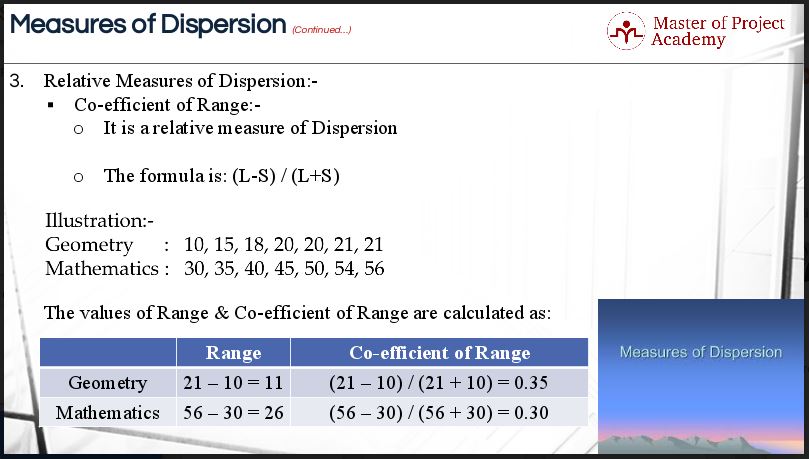
Let us take two sets of observations. Set A contains marks of seven students in Geometry out of 25 marks and group B contains marks of the same number of students in Mathematics out of 100 marks. We will need to calculate the range of marks in both subjects. In Geometry, the absolute range is 11, and in Mathematics, the absolute range is 26. This is based on absolute measures of dispersion, not relative measures of dispersion, but the reality is that the two subjects can not be compared directly as their base is not the same. When we convert these two values into coefficients of range, we see that the coefficient of range for Geometry is greater than that of Mathematics. Thus, there is greater dispersion or variation in Geometry. The marks of students in Mathematics are more stable than their marks in Geometry. We learn this using relative measures of dispersion.
Relative Measures of Dispersion: Coefficient of Quartile Deviation
How to calculate the coefficient of quartile deviation?
Let’s look at the example of the geometry and mathematics marks and use relative measures of dispersion to see the spread of the data regarding quartiles. We will now calculate the coefficient of quartile deviation for mathematics and geometry using the formula of quartile deviation, Q3 minus Q1 divided by Q3 plus Q1, and we see that the coefficient of quartile deviation for both Geometry and Mathematics is similar. It is 0.5 for both subjects. Therefore, the inference is that the marks or scores of students in both subjects indicate uniform median performance.
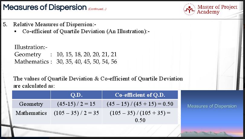
None of the subjects indicate higher or lower uniformity in median scores than each other. Please remember the fundamental rule about relative measures of dispersion here. When the coefficient of quartile deviation is small, it indicates high uniformity or fundamental rule about relative measures of dispersion here. When the coefficient of quartile deviation is small, it indicates high uniformity or a small variation of the central 50% items or high uniformity towards the median performance. When the coefficient of quartile deviation is high, it means the variation among the central 50% items is large, or uniformity in median performance is less. That was the second of the relative measures of dispersion.
Relative Measures of Dispersion: Coefficient of Variation
Let’s look at the last of the relative measures of dispersion. The type of the relative measures of dispersion that corresponds to standard deviation is the “Coefficient of Variation.” It is usually expressed in percentage terms and is the most commonly used of the relative measures of dispersion. Since relative measures of dispersion are free from the units in which the values have been expressed, they can be compared even across different groups having different units of measurement.
Inferences based on the coefficient of variance
Let us also talk about the method of drawing an inference. If we want to compare the variability of two or more groups or series of data, we can use the coefficient of variation. The series or groups of data, for which the coefficient of variation is greater, indicates that the group is more variable, less stable, less uniform, less consistent, or less homogeneous. If the coefficient of variation is lower, it indicates that the group is less variable, more stable, more uniform, more consistent, or more homogeneous. The formula for the coefficient of variation would be read as: sample standard deviation divided by sample mean multiplied by 100.
An example of calculating the coefficient of variance
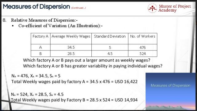
Please have a look at an illustration in the figures below. An example is about two factories: Factory A and Factory B which employ 476 and 524 workers respectively. The average weekly wages for each worker in Factory A and Factory B are USD 34.5 and USD 28.5 respectively. The standard deviation in paying the individual wages has been recorded as USD 5 and USD 4.5 for Factory A and Factory B respectively.
There are two questions here that we need to solve:
- Which factory A or B pays out a larger amount as average weekly wages?
- Which factory A or B has greater variability in paying individual wages?
Calculating average weekly wages
Let us first calculate which factory pays more amount of weekly wage than another. For the first factory, the numbers of workers are 476, the average weekly wages are USD 34.5, and the standard deviation is USD 5. Therefore, the amount of average weekly wages paid by Factory A is USD 34.5 multiplied by 476 is which is equal to USD 16,422. For the second factory, the numbers of workers are 524, the average weekly wages are USD 28.5, and the standard deviation is USD 4.5. Therefore, the amount of average weekly wages paid by Factory B is USD 28.5 multiplied by 524 which is equal to USD 14,934. It is now quite clear that Factory A pays a larger amount of weekly wages than Factory B.
Calculating the coefficient of variation in weekly wages
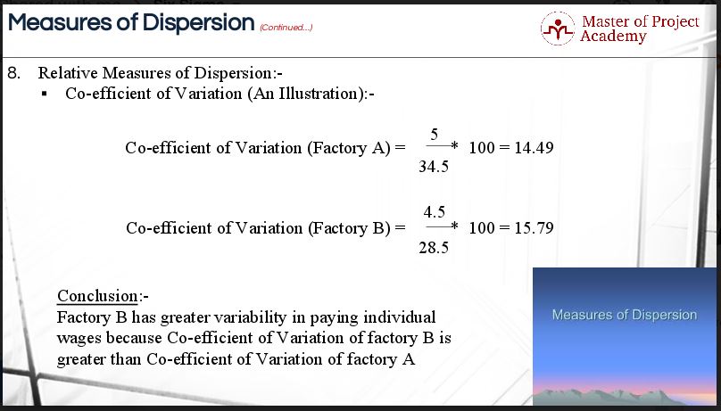
The next question asks which factory has greater variability in paying individual wages. For this purpose, we will have to calculate the coefficient of variation for both the factories. The formula for the coefficient of variation is: sample standard deviation divided by sample mean multiplied by 100. Therefore, the coefficient of variation for Factory A and Factory B is 14.49 and 15.79 respectively. The conclusion here is that Factory A has a lower coefficient of variation than Factory B. Factory A also pays more amount of average weekly wages than Factory B. Factory B has a higher coefficient of variation than Factory A. Therefore it indicates that the variability in the payment of individual wages is high. Factory B pays a lesser amount of average weekly wages than Factory A.
Inferences from the data
In Factory B, it can be estimated that a small chunk of workers takes away larger portions of wages because of internal irregularities or policies of the company or other reasons. The chances are that not every worker in Factory B earns the average amount of wages. However, this may not be the case with Factory A. That was the last of the relative measures of dispersion.
This simple example shows how relative measures of dispersion such as coefficient of variation can be used to draw inferences about sets of data, even if the data was measured in different units. Relative measures of dispersion are useful to Six Sigma teams for that reason as they can be confronted with many data sets with different units of measure. Just like absolute measures of dispersion, relative measures of dispersion are powerful tools to investigate the spread of observations in a dataset.