
In the Measure phase of the DMAIC process in Six Sigma, there are many types of statistical parameters that graduates of Lean Six Sigma Green Belt training or other Online Six Sigma courses should know. Measures of Central Tendency serve to locate the center of the distribution. However, they do not reveal how the items are spread out on either side of the center. To understand the spread of the data, Lean Six Sigma practitioners need to understand relative and absolute measures of dispersion. This characteristic of a frequency distribution is commonly referred to as ‘Dispersion’. The word ‘Dispersion’ refers to the lack of uniformity in the sizes or quantities of the items of a group or series of data. The word ‘Dispersion’ may also be used to indicate the spread of the data. It is a great way of showing how quantitative data is spread relative to the center point of the data.
Attend our 100% Online & Self-Paced Free Six Sigma Training.
Let’s have a detailed look at absolute measures of dispersion and how they are used in Six Sigma practices.
Dispersion and Uniformity
In a series of data, all the items or observations are not equal. There is a difference or variation among the values. The degree of variation is evaluated by various relative and absolute measures of dispersion. Small dispersion indicates high uniformity of the items, while large dispersion indicates less uniformity.
Absolute and Relative Measures of Dispersion Difference
There are two types of measures of dispersion, namely:
- Absolute measures of dispersion
- Relative measures of dispersion
Absolute measures of dispersion indicate the amount of variation in a set of values; in terms of units of observations. For example, when rainfall data is made available for different days in mm, any absolute measures of dispersion give the variation in rainfall in mm. On the other hand, relative measures of dispersion are free from the units of the measurements of the observations. They are pure numbers. They are used to compare the variation in two or more sets, which are having different units of measurements of observations. Both relative and absolute measures of dispersion are useful to Six Sigma teams.
Absolute Measures of Dispersion
The absolute measures of dispersion are as follows:
- Range
- Quartile deviation
- Mean deviation
- Standard deviation
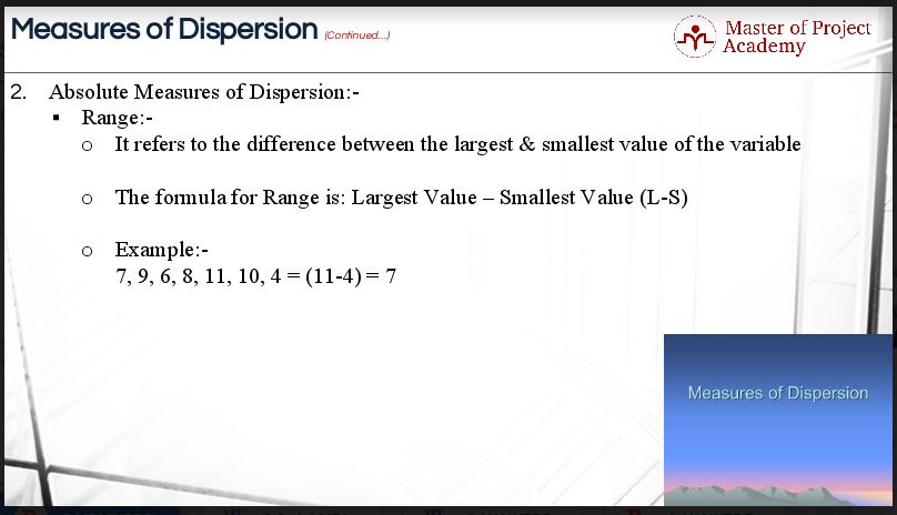
Range
This is the simplest possible of the absolute measures of dispersion and is defined as the difference between the largest and smallest values of the variable. The formula for range would be read as the largest value minus the smallest value. Symbolically, it is read as L minus S. Take a look at the simple illustration of the range in the figure below. The largest value in the data set is 11. The smallest value in the data set is 4. Hence; the range is 11 minus 4 and this makes 7. This is an example of one of the absolute measures of dispersion.
Absolute Measures of Dispersion: Quartile Deviation
What are Quartiles?
Before we move on to learn about one of the absolute measures of dispersion – quartile deviation, let’s think about what quartiles mean. Quartiles are the measures that divide the data into four equal parts; each portion contains an equal number of observations. Thus, there are three quartiles. The first quartile is denoted by Q1. It is also called as lower quartile. It has 25% of the items of the distribution below it and 75% of the items are greater than it. The second quartile is denoted by Q2. It is nothing but; the median of the data. It has 50% of items below it and 50% of the observations above it. The third quartile is denoted by Q3. It is also called as upper quartile. It has 75% of the items of the distribution below it and 25% of the items above it. Thus, Q1 and Q3 denote the two limits within which central 50% of the data lies. In other words, the third quartile minus the first quartile is equivalent to the medium of the data. That is it!
Absolute Measures of Dispersion: Quartile Deviation
In terms of absolute measures of dispersion, quartile deviation is half of the difference between the first and third quartiles, Q1 and Q3. Hence, it is also called the semi-inter quartile range because quartile deviation is equivalent to half of the inter-quartile range. When we talk about absolute measures of dispersion we usually stick to the term – quartile deviation.
Calculating the three quartiles
The first quartile, Q1, is equal to the size of N+1th divided by 4. In the case of the third quartile, Q3, simply multiply the formula for Q1 by 3. Therefore; the formula for quartile deviation is Q3 minus Q1 divided by 2.
Let us also try to understand the method of locating the second quartile. It is the same as that of the Median. Thus, the formula for Median will work here. The value of Q1 and Q3 can be obtained by the formula shown in the figure below where ‘N’ refers to the number of observations.
An illustration of the calculation of the three quartiles
The best way to understand how to calculate the quartile deviation as part of the absolute measures of dispersion is by illustration. Of course, absolute measures of dispersion can be calculated with appropriate software, but it is always good to understand the underlying arithmetics.
Take a look at the illustration of quartile deviation below. First of all, the values are arranged in ascending order. Once you do that, you will have to calculate the position of Q1. The formula for calculating Q1 is ‘n’ plus 1 divided by 4. So, ten plus one divided by 4 is equivalent to 2.75. The position of Q1 is equivalent to the value at the 2.75th position. We will have to calculate the value which lies at the 2.75th position. How do we do that? Here is the formula! Q1 will be equal to the value at the 2nd position plus 0.75 of the difference between the 3rd value and the 2nd value. The value at the 2nd and 3rd positions are 391 and 407 respectively. So, our equation will be 391 plus 0.75 of the difference between 407 and 391. The answer is 403. The Q1 is 403.
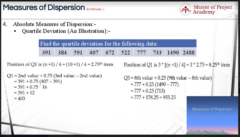
Calculate the position of Q3
Secondly; we will have to calculate the position of Q3. In order to arrive at the formula for calculating Q3, we simply need to multiply the formula for calculating Q1 by 3. The position of Q3 is equivalent to the value at the 8.25th position. We will have to calculate the value which lies at the 8.25th position. Q3 will be equal to the value at the 8th position plus 0.25 of the difference between the 9th value and 8th value. The value at the 8th and 9th positions is 777 and 1490 respectively. So, our equation will be 777 plus 0.25 of the difference between 1490 and 777. The answer is 955.25. The Q3 is 955.25.
Now, calculating the quartile deviation is very simple. The formula for calculating quartile deviation is Q3 minus Q1 divided by 2. Our Q3 and Q1 is equivalent to 955.25 and 403 respectively. Hence, the answer is 276.125. The quartile deviation in this problem is 276.125. This is how you calculate quartile deviation, one of the absolute measures of dispersion.
Standard Deviation
What is the standard deviation? The standard deviation plays a dominating role in the study of variation in the data. It is of great importance for the analysis of data and for the various statistical inferences.
The Standard Deviation is the the positive square root of the mean of the square deviations taken from arithmetic mean of the data.
In other words, the positive square root of the variance is the standard deviation. Please note that standard deviation is calculated on the basis of the mean or average only. The formula for sample standard deviation would be read as:
Square root of Summation of the bracket of square of X minus X-bar divided by the bracket of ‘n’ minus 1.
These three absolute measures of dispersion are most commonly used to describe the spread of the data around the center point. While the center of the data gives valuable insights, knowledge of the spread of the data completes the picture with absolute measures of dispersion and relative measures of dispersion. When Six Sigma teams collect data in the Measure phase of the DMAIC process, they will always look at the relative and absolute measures of dispersion to fully understand the data in front of them.