
Lean Six Sigma Green Belt course graduates deal with two types of data during the Six Sigma Measure phase of their Six Sigma DMAIC projects: continuous data and discrete data. The Poisson distribution is a probability distribution for discrete data which takes on the values which are X = 0, 1, 2, 3 and so on. As those who have completed an online Six Sigma training will know, the Poisson distribution characterizes data for which you can only count the nonconformities that exist.
Attend our 100% Online & Self-Paced Free Six Sigma Training.

The Poisson distribution characterizes defects data, which are also non-conformities that affect part of a product or service but that do not render the product or service unusable. Let’s see how the Poisson distribution works.
The History
The Poisson distribution was discovered by a French Mathematician-cum- Physicist, Simeon Denis Poisson in 1837. Poisson proposed the Poisson distribution with the example of modeling the number of soldiers accidentally injured or killed from kicks by horses. The Poisson distribution became useful as it models events, particularly uncommon events.
When to Use the Poisson Distribution?
The Poisson distribution is often used as a model for the number of events (such as the number of telephone calls at a business, the number of accidents at an intersection, number of calls received by a call center agent etc.) in a specific time period. The Poisson distribution is used when it is desired to determine the probability of the number of occurrences on a per-unit basis, for instance, per-unit time, per-unit area, per-unit volume etc. In other words, the Poisson distribution is the probability distribution that results from a Poisson experiment. The Poisson distribution is suitable for analyzing situations where the number of trials is very large and the probability of success is very small.
The Poisson Experiment
A Poisson experiment is a statistical experiment that has the following properties:
- The experiment results in outcomes that can be classified as successes or failures
- The average number of successes (μ) that occurs in a specified region is known
- The probability that a success will occur is proportional to the size of the region
- The probability that a success will occur in an extremely small region is virtually zero
The Poisson parameter Lambda (λ) is the total number of events (k) divided by the number of units (n) in the data The equation is: (λ = k/n).
The Formula
Have a look at the formula for Poisson distribution below.
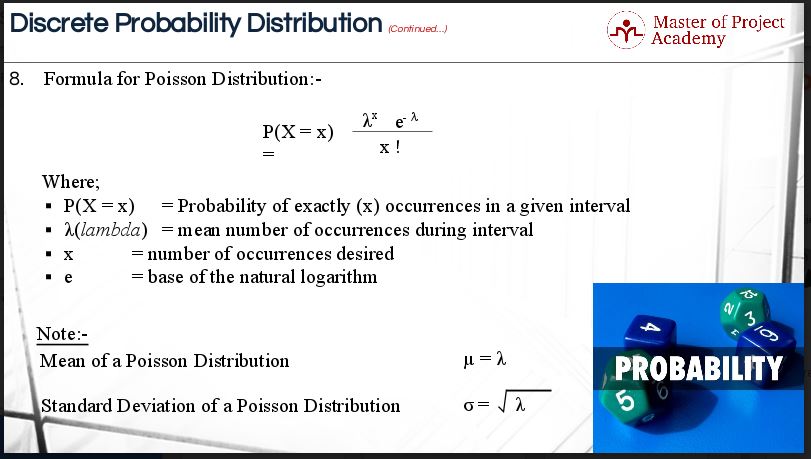
Let’s get to know the elements of the formula:
- P(X = x) refers to the probability of x occurrences in a given interval
- This symbol ‘ λ’ or lambda refers to the average number of occurrences during the given interval
- ‘x’ refers to the number of occurrences desired
- ‘e’ is the base of the natural algorithm. According to Poisson distribution table, the value of 0.0067 has been derived on the basis of the ‘λ’ value and ‘x’ value.
You can download the Poisson distribution table online.
An Illustration of Poisson distribution
The problem relates to the number of accidents at a dangerous signal. In order to investigate the efficiency of safety measures taken at a dangerous signal, it was decided to check past records. The records show that the average number of accidents every week at this signal is five. Since the number of accidents follows the Poisson distribution, we will calculate the probability of:
- Less than 2 accidents per week
- More than 3 accidents per week
Calculating probability of fewer than 2 accidents per week using the Poisson distribution
To answer the first point, we will need to calculate the probability of fewer than 2 accidents per week using Poisson distribution. Mathematically, it can be expressed as P (X< 2). The probability of less than 2 indicates the first possibility of zero accidents and the second possibility of one accident. Considering this aspect of probability, the formula has to be customized.
Since X refers to the number of occurrences desired, the preliminary equation has to be formed in such a manner that it mathematically expresses the result. Therefore, it is noted as ‘P(X = 0) + P(X = 1)’ The main component of the formula has been repeated twice for two segments of the result. The first segment is ‘P(X=0)’. The second segment is ‘P(X=1)’. The denominator in the main component of the formula mentions ‘0 Factorial’ and ‘1 Factorial’ and it has been expressed as 0 and 1 accompanied by an exclamation mark.
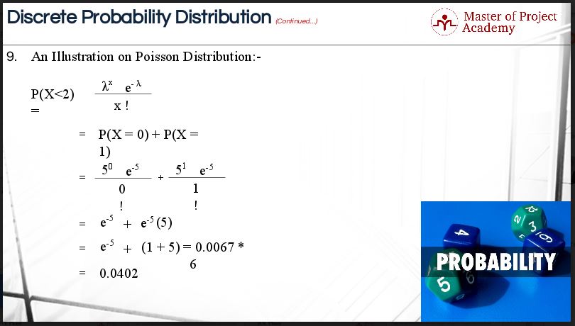
The numerator, for both the segments of the result, has the λ value of 5 for ‘x’ because the average number of historical accidents per week is five at the signal. ‘e’ is the base for the natural algorithm. We will need to refer Poisson distribution table to claim the value of algorithm. For the λ value of 5.0 and the row-wise ‘x’ value of ‘0’, the poison value is 0.0067 according to the Poisson distribution table. That is why the λ value of 0.0067 was provided in the example.
In this figure, the formula has further been solved. The algorithm value remains the same. Please note that 1 accident is the desired probability and 5 accidents are the historical average number. That is why the sum of one plus five has been multiplied by Poisson value. Therefore, the probability of fewer than 2 accidents per week is 0.0402 or 4.02%.
Calculating the probability of more than three accidents per week using the Poisson distribution
Now we will need to calculate the probability of more than 3 accidents per week using Poisson distribution. It can be expressed as ‘P (X >3)’. The probability of more than 3 indicates the first probability of zero accidents, the second probability of one accident, the third probability of two accidents and the fourth probability of 3 accidents. Considering this aspect of probability, the formula has to be customized.
Let us deep-dive into the formula one more time!
Since X refers to the number of occurrences desired, the preliminary equation has to be formed in such a manner that it expresses the result. Therefore, it is noted as ‘1 – {P(X = 0) + P(X = 1) + P(X = 2) + P(X = 3)}’. ‘1’ refers to 100% to account for limiting factor. The main component of the formula has been repeated four times for four segments of the result. The first segment is ‘P(X=0)’. The second segment is ‘P(X=1)’. The third segment is ‘P(X=2) and the fourth segment is ‘P(X=3)’.
The denominator in the main component of the formula mentions ‘0 Factorial’, ‘1 Factorial’, ‘2 Factorial’ and ‘3 Factorial’. It has been expressed as 0, 1, 2, and 3 accompanied with an exclamation mark. Please understand how factorial notation works. ‘2 factorial’ refers the value of ‘2*1 = 2’, ‘3 Factorial’ refers to the value of ‘3*2*1 = 6’.
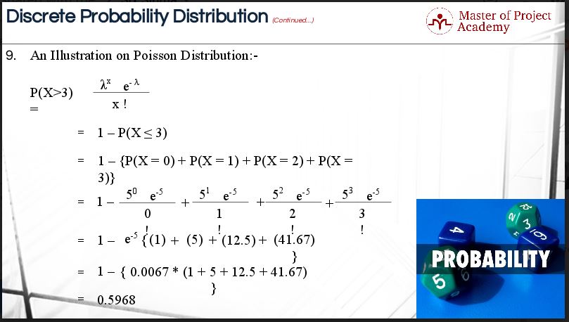
The numerator, for all the segments of the result, has the λ value of 5 for ‘x’ because the average number of historical accidents per week is five at the signal. For the λ value of 5.0 and the row-wise ‘x’ value of ‘0’, the poison value is 0.0067. It remains the same for calculating probability on both the occasions.
The formula has further been solved as normal. The common algorithm value has been noted outside the bracket. Note that 0 accidents, 1 accident, 2 accidents and 3 accidents are the desired probability and 5 accidents are the historical average number. That is why the sum of 1 plus 5 plus 12.5 plus 41.67 has been multiplied by Poisson value to be subtracted from 1 or 100%. Here we go with our answer. The probability of more than or equal to accidents per week is 0.5968 or 59.68%.
Calculating probability with the Poisson distribution may seem difficult at first, but once you get used to it, it’s actually very easy. What’s more, there are several software packages, like Minitab, which can do the Poisson distribution calculations for you! However, it is important to know how to calculate probability using the Poisson distribution by hand as well. As you can see, the Poisson distribution is very helpful in calculating the probability for discrete data.