
In the data-driven Six Sigma approach, it is important to understand the concept of probability distributions. Probability distributions tell us how likely an event is bound to occur. Different types of data will have different types of distributions. Why do we need to know this? Well, in the Lean Six Sigma Course we learn that probability distributions affect the types of statistical tools that are valid for that kind of data. So, when you have finished a reputable Lean training course and are able to apply Six Sigma practices, you will need to know what type of probability distribution is relevant to the data that you have collected during the Six Sigma Measure phase of your project’s DMAIC process.
Attend our 100% Online & Self-Paced Free Six Sigma Training.

What is Probability?
Let us first briefly understand what probability means. The word “probability” refers to a probable or likely event. Probability is a measure or estimation of how likely it is that something will happen or that a statement is true. Probabilities are given a value between 0 (0% chance or will not happen) and 1 (100% chance or will happen). The higher the degree of probability, the more likely the event is to happen, or, in a longer series of samples, the greater the number of times such event is expected to happen. In other words, the probability of an event is the measure of the chance that the event will occur as a result of an experiment.
How to calculate probability?
Probability is calculated by dividing the number of favorable outcomes by the total number of possible outcomes. The probability of a given event can be expressed in terms of ‘f’ divided by ‘N’. ‘f’ refers to the number of favorable outcomes and ‘N’ refers to the number of possible outcomes.
Three basic properties of probability
The three basic properties of Probability are as follows:
- Property 1: The probability of an event is always between 0 and 1, inclusive
- Property 2: The probability of an event that cannot occur is 0. Please note that an event that cannot occur is called an impossible event.
- Property 3: The probability of an event that must occur is 1. An event that must occur is called a certain event.
The simplest example is a coin flip. When you flip a coin there are only two possible outcomes, the result is either heads or tails. And so the probability of getting heads is 1 out of 2, or ½ (50%).

Probability Distribution Definition
Probability distribution maps out the likelihood of multiple outcomes in a table or an equation. In other words, it is a table or an equation that links each outcome of a statistical experiment with its probability of occurrence. To understand this concept, it is important to understand the concept of variables.
- A variable is a symbol (A, B, x, y, etc.) that can take on any of a specified set of values
- When the value of a variable is the outcome of a statistical experiment, that variable is called a random variable
Generally, statisticians use a capital letter to represent a random variable and a lower-case letter to represent different values in the following manner:
- X represents the Random Variable ‘X’
- P(X) represents the Probability of ‘X’
- P(X = x) refers to the probability that the random variable X is equal to a particular value, denoted by ‘x’. For example, P(X = 1) refers to the probability that the random variable X is equal to 1.
There are two main types of probability distribution: continuous probability distribution and discrete probability distribution. Today we will only be discussing the latter.
2 Types of Probability Distribution
What is discrete probability distribution?
A discrete probability distribution describes the probability of the occurrence of each value of a discrete random variable. A discrete random variable is a random variable that has countable values. The variable is said to be random if the sum of the probabilities is one.
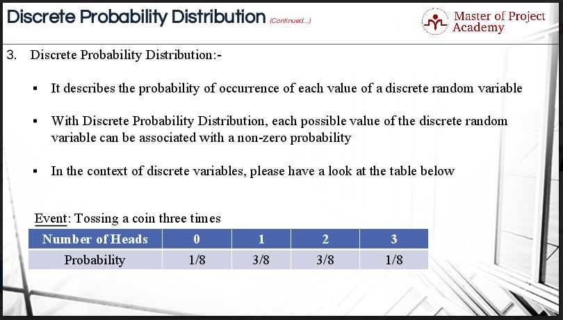
For example, if a coin is tossed three times, then the number of heads obtained can be 0, 1, 2 or 3. In other words, the number of heads can only take 4 values: 0, 1, 2, and 3 and so the variable is discrete. Note that getting either a heads or tail, even 0 times, has a value in a discrete probability distribution.
An example of discrete probability distribution
Now, have a look at the table in the figure below. The sum of all probabilities is equal to one. If the number of heads can take 4 values, then the number of tails can also take 4 values. The sum total is noted as a denominator value. That is why the probability result is one by eight. With a discrete probability distribution, each possible value of the discrete random variable can be associated with a non-zero probability. Thus, a discrete probability distribution is often presented in tabular form.
What is uniform probability distribution?
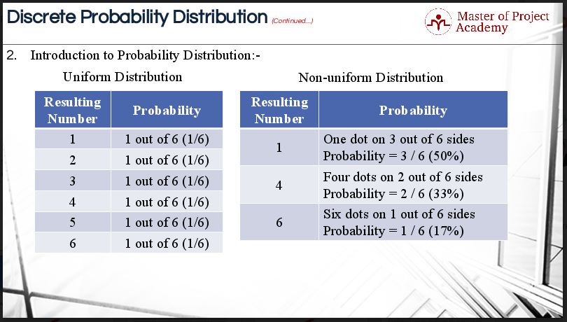
Please have a look at the table regarding uniform probability distribution in the figure below. Here’s an example to help clarify the concept. It relates to rolling a dice. A fair die has six sides, each side numbered from 1 to 6 and each side is equally likely to turn up when rolled. A probability distribution can be compiled like that of the uniform probability distribution table in the figure, showing the probability of getting any particular number on one roll.
Let us continue with the same example to understand non-uniform probability distribution. We will have to assume that we have modified a die so that three sides had 1 dot, two sides had 4 dots and one side had 6 dots. Now, there are only three possible number outcomes (1, 4 and 6) and the probability of getting each of these numbers is different. Please refer the table for non-uniform distribution in the figure to see the example.
There are two main types of discrete probability distribution: binomial probability distribution and Poisson probability distribution. We will not be addressing these two discrete probability distributions in this article, but be sure that there will be more articles to come that will deal with these topics. Now that you know what discrete probability distribution is, you can use them to understand your Six Sigma data.