Six Sigma is a data-driven approach to problem-solving. The six Sigma approach involves many statistical and mathematical concepts such as the normal distribution curve. Lean Six Sigma courses discuss the main statistical concepts necessary to solve problems according to 6 sigma rules. Six Sigma principles rely heavily on the understanding of the normal distribution curve as briefly discussed in online free Six Sigma courses. Let’s have a look at what a normal distribution curve means.
What is the normal distribution curve?
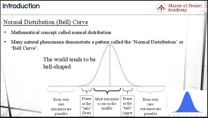
The term “Normal Distribution Curve” or “Bell Curve” is used to describe the mathematical concept called normal distribution, sometimes referred to as Gaussian distribution. It refers to the shape that is created when a line is plotted using the data points for an item that meets the criteria of ‘Normal Distribution’.
Attend our 100% Online & Self-Paced Free Six Sigma Training.

Natural phenomena follow a normal distribution curve
Many natural phenomena demonstrate a pattern called the ‘Normal Distribution Curve’ or ‘Bell Curve’. If you measure the height of women across the world, the results will follow a predictable form that resembles the bell shape. Temperature also follows this pattern. If you measure the average noon temperature for July days in the US each year, you would find that the observations followed a bell curve pattern. You could also try to measure the height of all your colleagues at work, or the time they take to drink a cup of coffee and you will find approximately normal distributions.
The structure of a normal distribution curve
Let’s look at the structure of a normal distribution curve. The center contains the value where the value of the greatest number of data points occurs and therefore would be the highest point on the arc of the line. This point of the normal distribution curve is the mean or average. To use the example of height, there will be more instances of women of average height than any other height, therefore, the value of the average height of women in the world will be at the top of the normal distribution curve.
The mean, median, and mode of a normal distribution curve
Please note that in the case of normally distributed data, the mean will be equal to both the median and the mode. Let’s review the difference between the mean, median, and mode. The mean is the sum of all the values of the data points divided by the number of data points. If you line up all the values from smallest to largest, the middle value will be the median. In contrast, the mode is the number that appears most often in a set of data points. In a normal distribution, the mean, the median, and the mode will be the same.
Outliers in a normal distribution
The normal distribution curve is concentrated in the center and decreases on either side. This is significant as the data tends to have fewer incidences of unusually extreme values, called outliers or special causes of variation (SCV), as compared to other distributions. Because the data set has few extreme numbers on either the lower or the higher end of the scale, the curve flattens. This is what gives the normal distribution curve its bell-like shape.
Normal distributions in terms of means and standard deviations
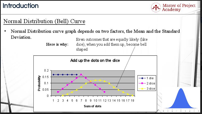
Let’s look at the shape of a normal distribution curve from another angle. A curve graph depends on two factors, the mean and the standard deviation. Let’s quickly review the definition of standard deviation. The standard deviation is a measure of how closely grouped or how widely spaced a set of data appears. It is one of the measures of dispersion. A standard normal distribution has a mean of zero and a standard deviation of one. The mean identifies the position of the center and the standard deviation determines the height and width of the bell.
For example, a large standard deviation creates a flat and wide-shaped bell while a small standard deviation creates a narrow and steeper curve. The rule is simple. The flatter the curve, the higher the variation. The steeper the curve, the lower the variation.
A practical example of the normal distribution curve
Let’s go over an example in this figure below:
- If you roll a single die, the possibility of each number to be rolled is around 16.67% for each number.
- If you roll two dice, the possibility of the sum of the dots will be as shown in the pink line. It will be from 2 to 12 respectively. But as you see, the possibility of getting the sum as 7 is the highest, which is actually 2 plus 12 divided by 2.
- Finally, if you roll three dice at the same time, the possibility of the sum of the dots will be as shown in the yellow line. The result will be ranging from 3 to 18. But as you see, the possibility of getting the sum as 10 or 11 is the highest, which is actually close to 10.5, and this is if found by 3 plus 18 divided by 2.
Now, let’s also recall the empirical rule of standard deviation. It says that within a standard normal distribution:
- 68% of the data points will fall within ± one standard deviation from the mean
- 95% will fall within ± two standard deviations
- 99.73% of the data points will fall within ± three standard deviations from the mean
Let’s summarize: The normal distribution curve is a probability distribution where the most frequently occurring value is in the middle and other probabilities tail off symmetrically in both directions. So distribution is symmetric.
- Theoretically, it does not reach zero
- The normal distribution curve can be divided in half with equal values falling on either side Of the most frequently occurring value
- Indicates random variable or chance variation
- The peak of the normal distribution curve represents the center of the process
- They are divided up into 3 standard deviations on each side of the mean
The normal distribution curve is one of the most important statistical concepts in Lean Six Sigma. Lean Six Sigma solves problems where the number of defects is too high. A high number of defects statistically equals high variation in the process. The normal distribution curve visualizes the variation in a data set. The data set represented by the curve could refer to downtime in manufacturing or the amount of time it takes to take a call in a call center. If the data follows a normal distribution curve, it means that the data is eligible for certain statistical tests that are used in the analyze stage of the Six Sigma process.